Spatial data & visualization

Introduction to Data Science

introds.org

1854 London Cholera Outbreak

2013 - 2018 West Nile virus spread

Map generated from nextstrain.org

2013 - 2018 West Nile virus spread

Map generated from nextstrain.org

Many others!

Spatial data is different

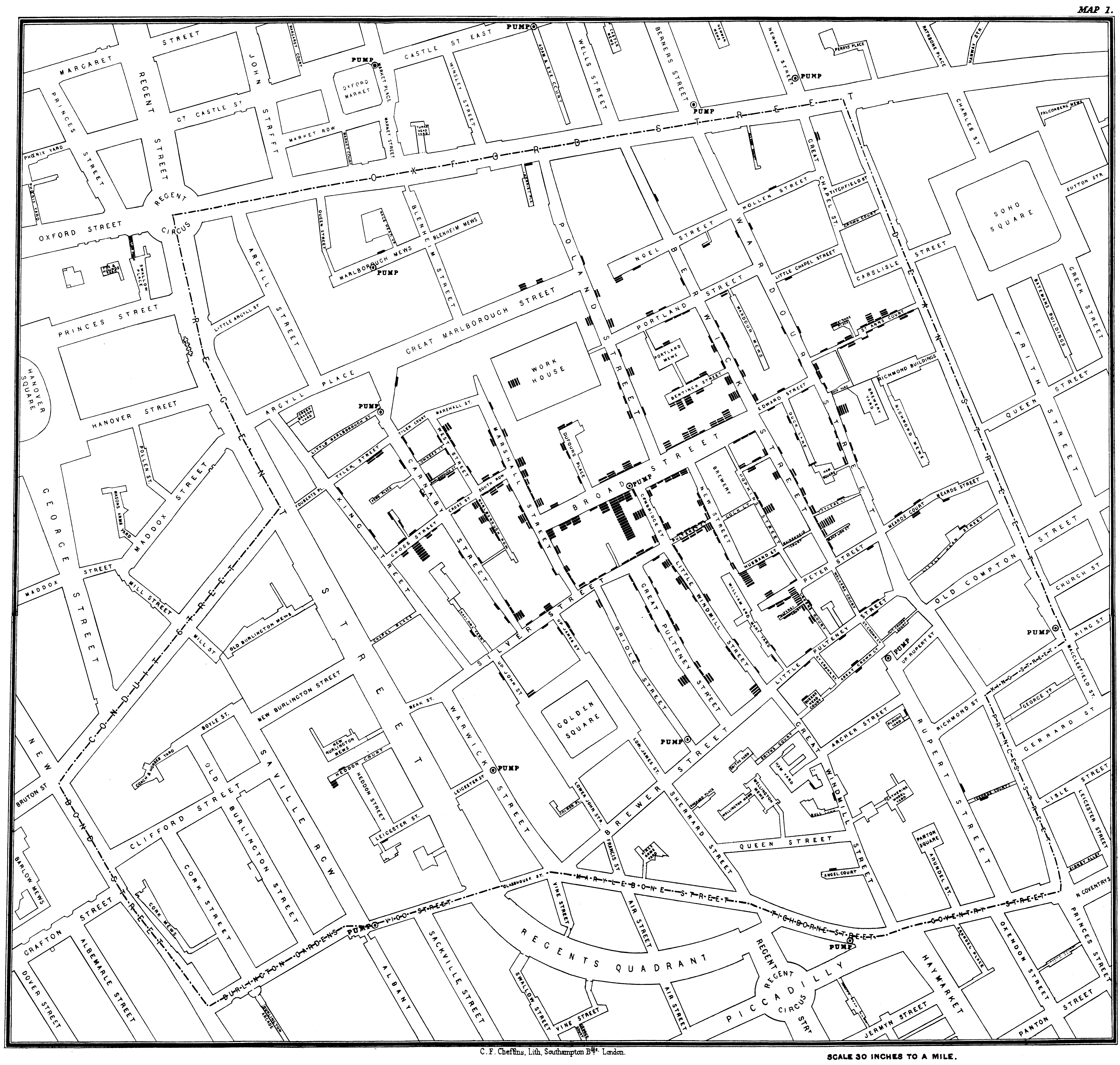
Our typical tidy data frame:

## # A tibble: 336,776 × 19
##     year month   day dep_time sched_dep_time dep_delay arr_time sched_arr_time
##    <int> <int> <int>    <int>          <int>     <dbl>    <int>          <int>
##  1  2013     1     1      517            515         2      830            819
##  2  2013     1     1      533            529         4      850            830
##  3  2013     1     1      542            540         2      923            850
##  4  2013     1     1      544            545        -1     1004           1022
##  5  2013     1     1      554            600        -6      812            837
##  6  2013     1     1      554            558        -4      740            728
##  7  2013     1     1      555            600        -5      913            854
##  8  2013     1     1      557            600        -3      709            723
##  9  2013     1     1      557            600        -3      838            846
## 10  2013     1     1      558            600        -2      753            745
## # … with 336,766 more rows, and 11 more variables: arr_delay <dbl>,
## #   carrier <chr>, flight <int>, tailnum <chr>, origin <chr>, dest <chr>,
## #   air_time <dbl>, distance <dbl>, hour <dbl>, minute <dbl>, time_hour <dttm>

Spatial data is different

Our (new) simple feature object:

## Simple feature collection with 100 features and 3 fields
## Geometry type: MULTIPOLYGON
## Dimension:     XY
## Bounding box:  xmin: -84.32385 ymin: 33.88199 xmax: -75.45698 ymax: 36.58965
## Geodetic CRS:  NAD27
## First 10 features:
##           name regstrd voted                       geometry
## 1         ASHE   19414  8428 MULTIPOLYGON (((-81.47276 3...
## 2    ALLEGHANY    7556  4101 MULTIPOLYGON (((-81.23989 3...
## 3        SURRY   46666 23660 MULTIPOLYGON (((-80.45634 3...
## 4    CURRITUCK   21803  7536 MULTIPOLYGON (((-76.00897 3...
## 5  NORTHAMPTON   13891  6196 MULTIPOLYGON (((-77.21767 3...
## 6     HERTFORD   14945  6955 MULTIPOLYGON (((-76.74506 3...
## 7       CAMDEN    8128  3472 MULTIPOLYGON (((-76.00897 3...
## 8        GATES    8294  3105 MULTIPOLYGON (((-76.56251 3...
## 9       WARREN   13441  6878 MULTIPOLYGON (((-78.30876 3...
## 10      STOKES   31649 14444 MULTIPOLYGON (((-80.02567 3...

Raster versus vector spatial data

Vector spatial data describes the world using shapes (points, lines, polygons, etc).

Raster spatial data describes the world using cells of constant size.

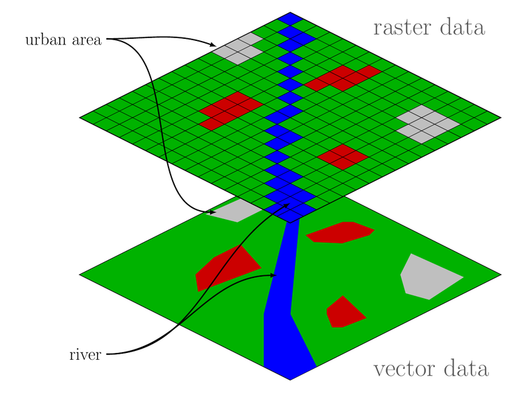
Source: https://commons.wikimedia.org/wiki/File:Raster_vector_tikz.png

Simple features

A simple feature is a standard way to describe how real-world spatial objects (country, building, tree, road, etc) can be represented by a computer.

Simple features

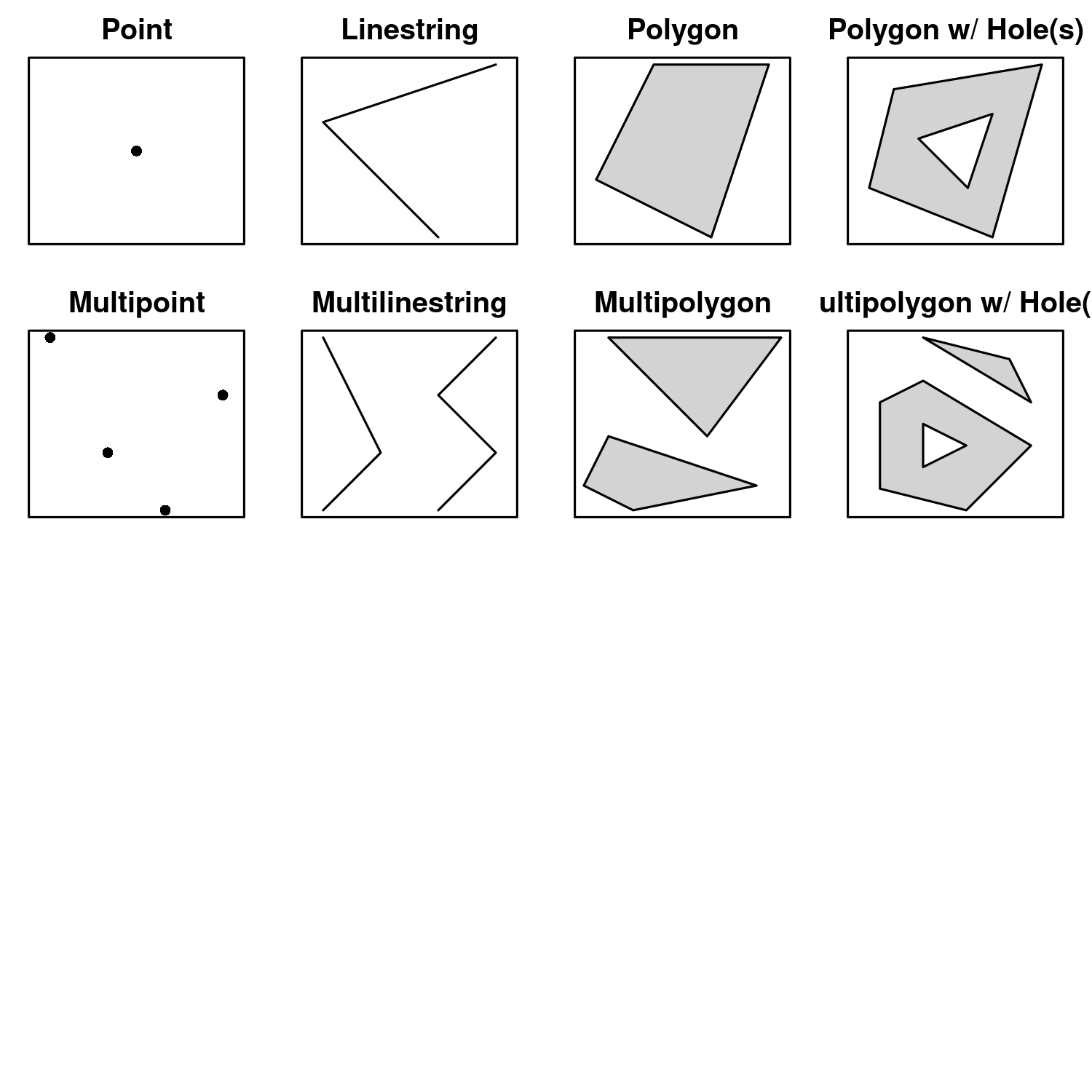
A simple feature is a standard way to describe how real-world spatial objects (country, building, tree, road, etc) can be represented by a computer.

The package sf implements simple features and other spatial functionality using tidy principles.

Simple features

Simple features have a geometry type. Common choices are below.

A simple feature objectSimple features are stored in a data frame, with the geographic information 
in a column called geometry.
Simple features can contain both spatial and non-spatial data.
Functions for spatial data in sf begin st_.
9

Visualizing spatial data10

`nc_votes`

This data is from the North Carolina Early Voting Statistics website, October 2020.

The dataset contains the following variables:

name: county name
regstrd: number of registered voters
voted: number of individuals who have voted
mailed: number of mail ballots returned
rejectd: number of mail ballots rejected
ml_rqst: number of mail ballots requested

Getting `sf` objects

To read simple features from a file or database use the function st_read().

library(sf)
nc <- st_read("data/nc_votes.shp", quiet = TRUE)
nc

## Simple feature collection with 100 features and 6 fields
## Geometry type: MULTIPOLYGON
## Dimension:     XY
## Bounding box:  xmin: -84.32385 ymin: 33.88199 xmax: -75.45698 ymax: 36.58965
## Geodetic CRS:  NAD27
## First 10 features:
##           name regstrd voted mailed rejectd ml_rqst
## 1         ASHE   19414  8428     NA      NA    2666
## 2    ALLEGHANY    7556  4101     NA      NA     971
## 3        SURRY   46666 23660   4366       7    7088
## 4    CURRITUCK   21803  7536     NA      NA    2472
## 5  NORTHAMPTON   13891  6196    828       2    1441
## 6     HERTFORD   14945  6955     NA      NA    1524
## 7       CAMDEN    8128  3472    416       1     739
## 8        GATES    8294  3105     NA      NA     847
## 9       WARREN   13441  6878     NA      NA    1913
## 10      STOKES   31649 14444   2162       2    3648
##                          geometry
## 1  MULTIPOLYGON (((-81.47276 3...
## 2  MULTIPOLYGON (((-81.23989 3...
## 3  MULTIPOLYGON (((-80.45634 3...
## 4  MULTIPOLYGON (((-76.00897 3...
## 5  MULTIPOLYGON (((-77.21767 3...
## 6  MULTIPOLYGON (((-76.74506 3...
## 7  MULTIPOLYGON (((-76.00897 3...
## 8  MULTIPOLYGON (((-76.56251 3...
## 9  MULTIPOLYGON (((-78.30876 3...
## 10 MULTIPOLYGON (((-80.02567 3...

Plotting with `ggplot()`

ggplot(nc) +
  geom_sf() +
  labs(title = "North Carolina counties")

A look at some aesthetics

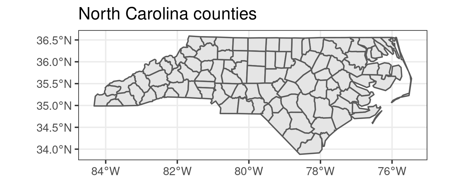
ggplot(nc) +
  geom_sf(color = "green") +
  labs(title = "North Carolina counties with theme and aesthetics")

A look at some aesthetics

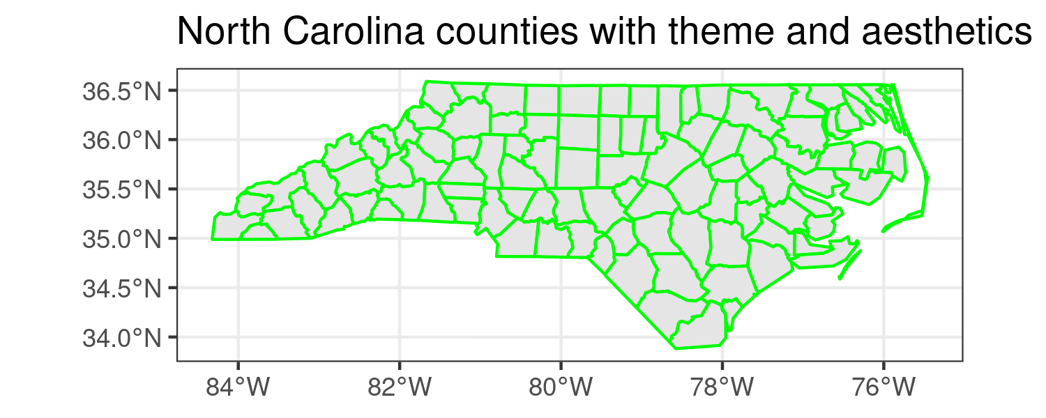
ggplot(nc) +
  geom_sf(color = "green", size = 1.5) +
  labs(title = "North Carolina counties with theme and aesthetics")

A look at some aesthetics

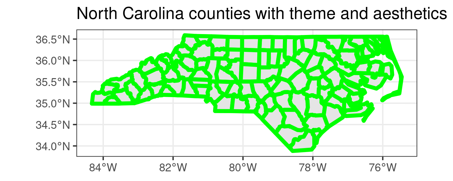
ggplot(nc) +
  geom_sf(color = "green", size = 1.5, fill = "purple") +
  labs(title = "North Carolina counties with theme and aesthetics")

A look at some aesthetics

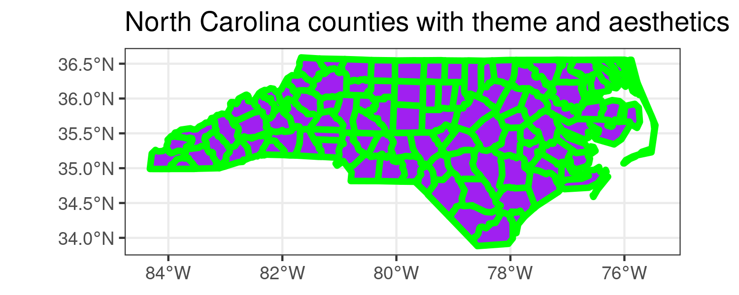
ggplot(nc) +
  geom_sf(color = "green", size = 1.5, fill = "purple", alpha = 0.50) +
  labs(title = "North Carolina counties with theme and aesthetics")

A look back at some of our data

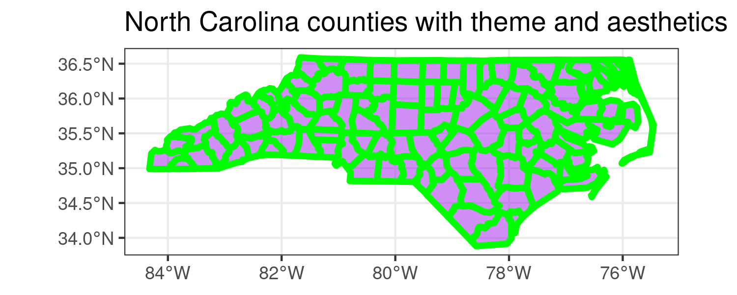
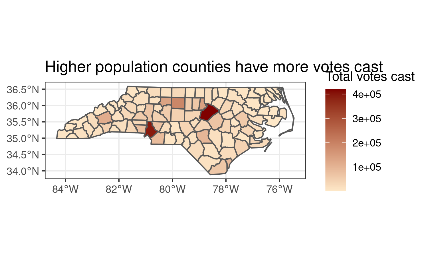
## Simple feature collection with 100 features and 6 fields
## Geometry type: MULTIPOLYGON
## Dimension:     XY
## Bounding box:  xmin: -84.32385 ymin: 33.88199 xmax: -75.45698 ymax: 36.58965
## Geodetic CRS:  NAD27
## First 10 features:
##           name regstrd voted mailed rejectd ml_rqst
## 1         ASHE   19414  8428     NA      NA    2666
## 2    ALLEGHANY    7556  4101     NA      NA     971
## 3        SURRY   46666 23660   4366       7    7088
## 4    CURRITUCK   21803  7536     NA      NA    2472
## 5  NORTHAMPTON   13891  6196    828       2    1441
## 6     HERTFORD   14945  6955     NA      NA    1524
## 7       CAMDEN    8128  3472    416       1     739
## 8        GATES    8294  3105     NA      NA     847
## 9       WARREN   13441  6878     NA      NA    1913
## 10      STOKES   31649 14444   2162       2    3648
##                          geometry
## 1  MULTIPOLYGON (((-81.47276 3...
## 2  MULTIPOLYGON (((-81.23989 3...
## 3  MULTIPOLYGON (((-80.45634 3...
## 4  MULTIPOLYGON (((-76.00897 3...
## 5  MULTIPOLYGON (((-77.21767 3...
## 6  MULTIPOLYGON (((-76.74506 3...
## 7  MULTIPOLYGON (((-76.00897 3...
## 8  MULTIPOLYGON (((-76.56251 3...
## 9  MULTIPOLYGON (((-78.30876 3...
## 10 MULTIPOLYGON (((-80.02567 3...

Let's incorporate these variables into our plot using ggplot.

Choropleth map

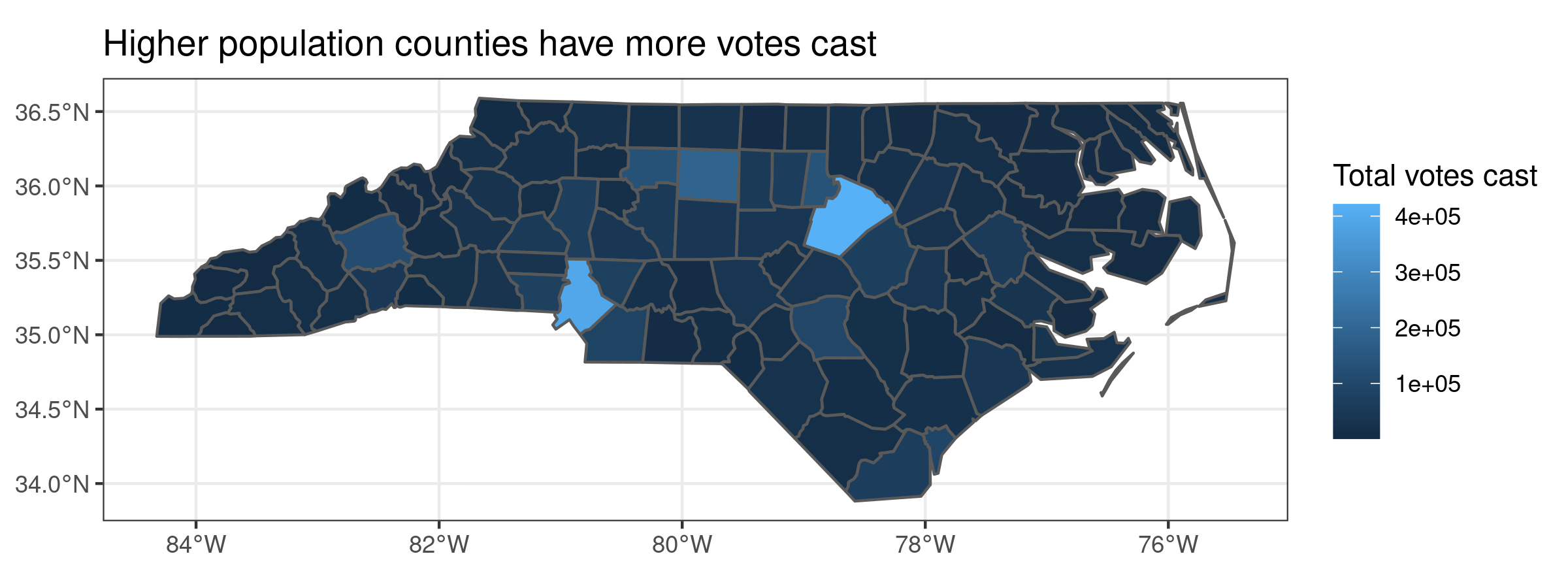
ggplot(nc) +
  geom_sf(aes(fill = voted)) +
  labs(title = "Higher population counties have more votes cast",
       fill = "Total votes cast")

It is sometimes helpful to pick diverging colors, colorbrewer2 can help.

Choropleth map

One way to set fill colors is with scale_fill_gradient().

ggplot(nc) +
  geom_sf(aes(fill = voted)) +
  scale_fill_gradient(low = "#fee8c8", high = "#7f0000") +
  labs(title = "Higher population counties have more votes cast",
       fill = "Total votes cast")

"...it's just a population map!"

Let's make it more informative

ggplot(nc) +
  geom_sf(aes(fill = voted/regstrd)) +
  scale_fill_gradient(low = "#fff7f3", high = "#49006a") +
  labs(fill = "Votes cast per registered voter", 
       title = "Early vote turnout varies by county")

Map layers23

Game Lands data

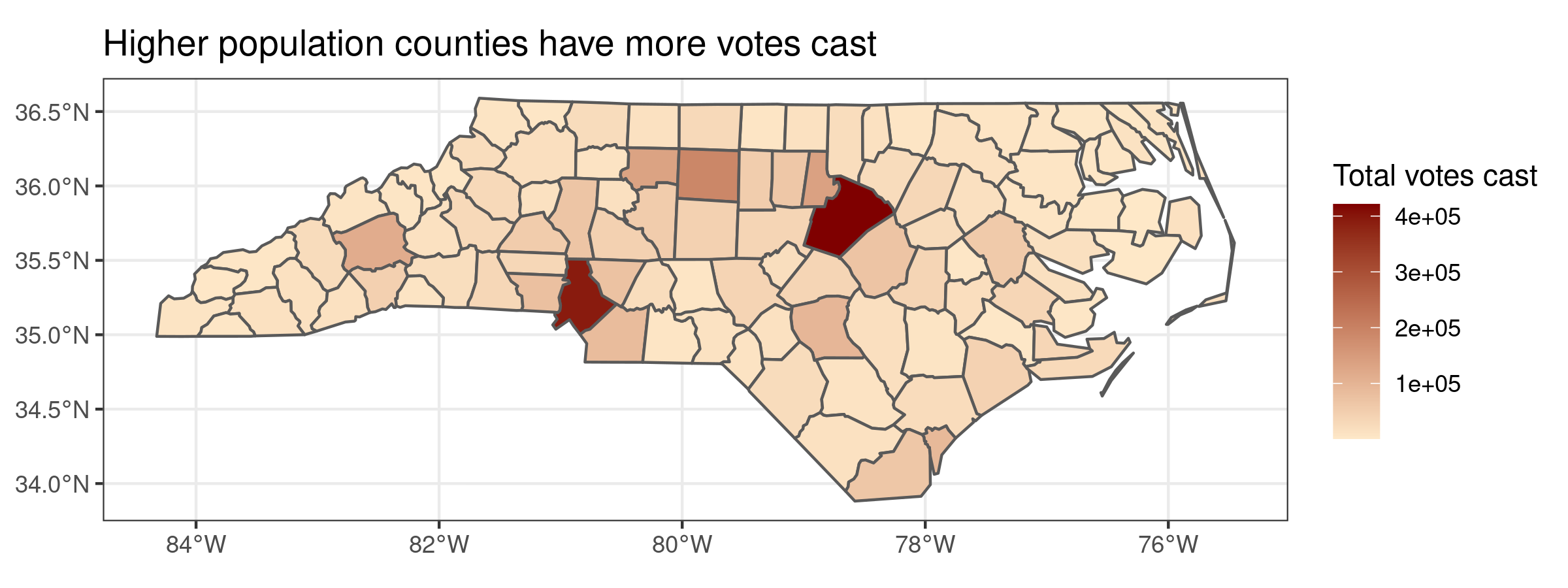
The North Carolina Department of Environment and Natural Resources, Wildlife Resources Commission and the NC Center for Geographic Information and Analysis has a shapefile data set available on all public Game Lands in NC.

nc_game <- st_read("data/gamelands.shp", quiet = TRUE)

A closer looknc_game

## Simple feature collection with 94 features and 6 fields
## Geometry type: MULTIPOLYGON
## Dimension:     XY
## Bounding box:  xmin: -84.29534 ymin: 33.98542 xmax: -75.54947 ymax: 36.58814
## Geodetic CRS:  NAD27
## First 10 features:
##    OBJECTID                   GML_HAB  SUM_ACRES GameLandID Shape__Are
## 1         1                     Alcoa 11395.9471          1   69931121
## 2         2           Alligator River 24439.0891          2  151120825
## 3         3                Angola Bay 34063.4468          3  204400526
## 4         4              Bachelor Bay  2786.2577          4   17219484
## 5         5             Bertie County  3883.7683          5   24044312
## 6         6 Bladen Lakes State Forest 33671.8426          6  202085696
## 7         7             Brinkleyville  1843.8439         92   11511489
## 8         8                  Buckhorn   491.3477         81    3046371
## 9         9                 Buckridge 17965.7187         10  110580903
## 10       10              Buffalo Cove  6630.9453         11   41161465
##    Shape__Len                       geometry
## 1   549030.42 MULTIPOLYGON (((-80.07347 3...
## 2   186792.83 MULTIPOLYGON (((-76.11832 3...
## 3   105421.80 MULTIPOLYGON (((-77.86947 3...
## 4    32891.84 MULTIPOLYGON (((-76.73896 3...
## 5    83468.94 MULTIPOLYGON (((-76.9209 35...
## 6   255198.44 MULTIPOLYGON (((-78.46171 3...
## 7    46838.19 MULTIPOLYGON (((-77.90555 3...
## 8    13445.00 MULTIPOLYGON (((-79.22056 3...
## 9   142923.83 MULTIPOLYGON (((-76.10961 3...
## 10   98754.34 MULTIPOLYGON (((-81.53307 3...
25

Visualize `nc_game`

ggplot(nc_game) +
  geom_sf() +
  labs(title = "North Carolina gamelands")

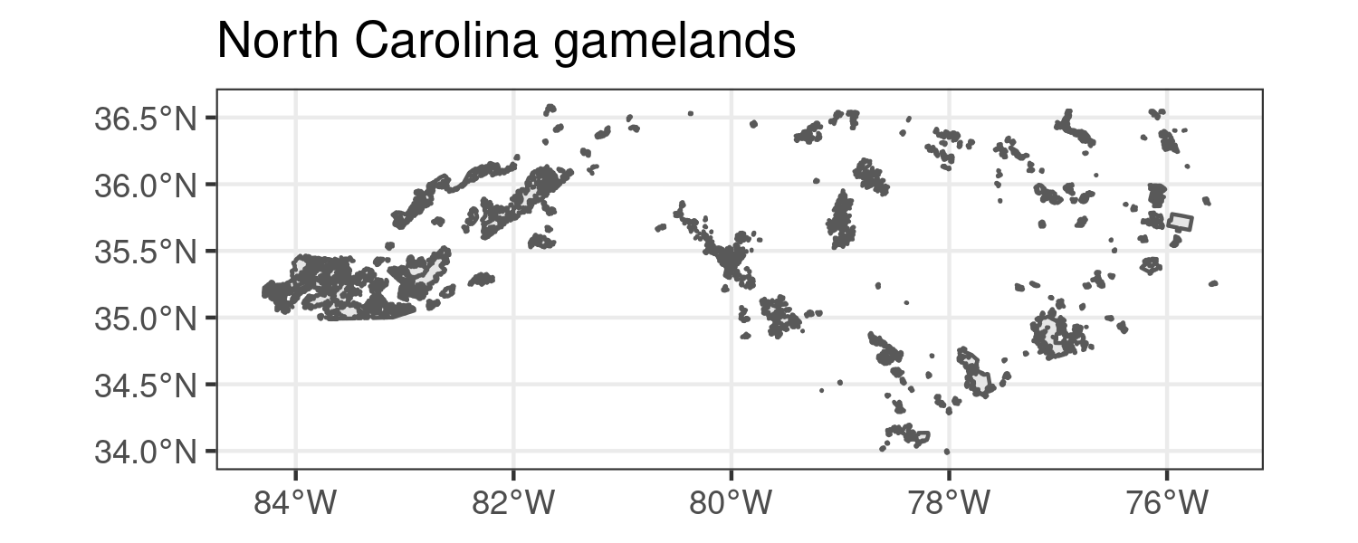
Visualize `nc_game`

ggplot(nc_game) +
  geom_sf(fill = "#ff6700") +
  labs(title = "North Carolina gamelands")

Add layers

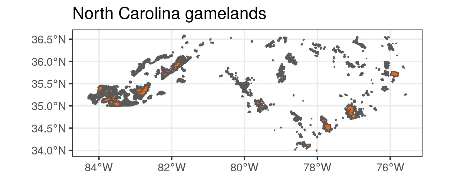
ggplot(nc) +
  geom_sf() +
  geom_sf(data = nc_game, fill = "#ff6700", alpha = .5) +
  labs(title = "North Carolina gamelands and counties")

Add layers and aesthetics

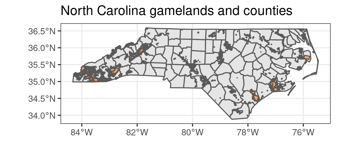
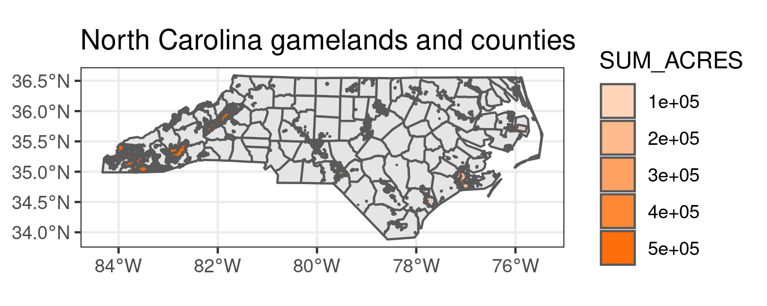
ggplot(nc) +
  geom_sf() +
  geom_sf(data = nc_game, aes(alpha = SUM_ACRES), fill = "#ff6700") +
  labs(title = "North Carolina gamelands and counties")

Spatial challenges30

Challenge #1

Different types of data exist (raster and vector).

Challenge #2

The coordinate reference system (CRS) matters.

```r
Simple feature collection with 100 features and 1 field
geometry type:  MULTIPOLYGON
dimension:      XY
bbox:           xmin: -84.32385 ymin: 33.88199 xmax: -75.45698 ymax: 36.58965
epsg (SRID):    4326
proj4string:    +proj=longlat +datum=WGS84 +no_defs
# A tibble: 100 x 2
  NAME                                                geometry
  <chr>                                     <MULTIPOLYGON [°]>
1 Ashe        (((-81.47276 36.23436, -81.54084 36.27251,  -...
```

Challenge #3

Manipulating spatial data objects is similar, but not identical to manipulating data frames.

Note the core data-wrangling functions from dplyr do work.

References

Help

Keyboard shortcuts

↑, ←, Pg Up, k

Go to previous slide

↓, →, Pg Dn, Space, j

Go to next slide

Home

Go to first slide

End

Go to last slide

Number + Return

Go to specific slide

b / m / f

Toggle blackout / mirrored / fullscreen mode

Clone slideshow

Toggle presenter mode

Restart the presentation timer

?, h

Toggle this help

Spatial data & visualization

Introduction to Data Science

introds.org

1854 London Cholera Outbreak

2013 - 2018 West Nile virus spread

2013 - 2018 West Nile virus spread

Spatial data is different

Spatial data is different

Raster versus vector spatial data

Simple features

Simple features

Simple features

A simple feature object

Visualizing spatial data

nc_votes

Getting sf objects

Plotting with ggplot()

A look at some aesthetics

A look at some aesthetics

A look at some aesthetics

A look at some aesthetics

A look back at some of our data

Choropleth map

Choropleth map

"...it's just a population map!"

Let's make it more informative

Map layers

Game Lands data

A closer look

Visualize nc_game

Visualize nc_game

Add layers

Add layers and aesthetics

Spatial challenges

Challenge #1

Challenge #2

Challenge #3

References

1854 London Cholera Outbreak

Help

`nc_votes`

Getting `sf` objects

Plotting with `ggplot()`

Visualize `nc_game`

Visualize `nc_game`